HIV and the Immune System - A Mathematical Model
Amstetten, Lower Austria
Abstract
| We
discuss a mathematical model of increasing the HI-viruses in the human
body. This model gives an answer to the question why the space of
time between HI-infection and outbreak of AIDS differs to a great
extent. It also gives insight into the phenomenon that our immune
system is generally not able to root out HI-viruses completely. This example is interesting from different view points:It is well suited for lessons combining subjects like mathematics and biology. It demonstrates that even extensive simulations can be well done by the TI92/TI89 or DERIVE. It emphasizes the usefullness of recursively defined sequencies which prove to be a multifunctional tool. |
The starting point of the model to be discussed is the increase of HI-viruses in the human body. This model gives an answer to the question why the space of time between HIVinfection and outbreak of AIDS differs to a great extent. Whereas some of the concerned die within months after infection, others ( but only a rather small number) are still alive without any troubles even 20 years later. After about 10 years half of all the infected suffer from AIDS. The following model - mainly developed by the Austrian mathematician M.Nowak - gives also insight into the phenomenon that our immune system is generally not able to root out HI-viruses completely as it is able to do with other types of viruses.
A paradox result of this model is the evidence that HI-viruses are that „successfull„ because their replication is susceptible to mistakes. As the transcription of virus-RNA to DNA is regularly connected with random mistakes, the likelyhood for a completely correct transmission of the genetic information is only about 40 percent.
Against every mutated
virus the immune system must create new specific killer cells, which can
only fight this special kind. The resistant cells act as specialists.
On the contrary all mutating viruses can destroy all kinds of resistant
cells against HIV or at least impair their function. The work as generalists.
In a tough fight against steadily appearing new kinds of AIDS-agents,
which are generated in the body of the infected person, the immunse system
is not able to work as efficiently as it should to maintain the balance.
If a certain variety of viruses is exceeded, the immune system finally
loses control of them and AIDS breaks out. In this way the number of virus-paricels
increases sharply whereas the number of immune cells drastically decreases.
[NOWAK, 1992]
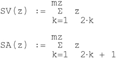
According to [LIPPA, 1997 bzw. REICHEL, 1999] the number vj(i) of the viruses of the kind i, j steps of time after infection can be described by means of the following (iterative) equation:
Here the factor of proportionality K describes the increase of the kind i of the resistant cells, which is generated by the mutant i of the viruses. The factor U characterises the aggressiveness of the viruses.
By analogy it is: 0<U<1. The term vj describes the total number of all viruses after j steps of time.
- First of all the number of mutants is unknown. In the simplest case this number is 1.This case shows the effect of the resistant cells well, but cannot explain the breakout of AIDS. Using relatively realistic parameters there are 11 mutants, resulting in at least 22 difference equations.
- In every step of
iteration the total number of viruses vj must be calculated.
The (iterative) equations, which describe the development of the various
types of viruses ( and consequentely the ones of the (iterativ) equations
of the resistant cells) are combined by the term

- The number of virus mutants as well as the kind and time of their appearance shall be controlled in this simulation.
- The more (iterative) equations (difference equations) are used the higher the likelyhood of mistakes and the less useful the simulation for application at school. Therefore it is decisive that the model remains applicable. Supporting programs or utility files, which create the respective equations automatically, prove to be a practicable way.
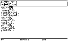
| R=0,1 / P=0,002
/ K=0,02 / U=0,00004 One step in time represents 0,005 years (i.e. 200 steps describe a year). In this example there are M=5000 cells in the reviewed volume of body liquid. The treshold value for the outbreak of AIDS is in this case 11 mutants, the limit for the total number of immune cells is 500. |
The sequence-mode
of TI-92 allows the direct input of the respective equations of the model.
The names of the equations are determined by u1,u2,u3, ... in this calculating
system. In our case u1(n) is the number of viruses of type 1 after n
steps of time, u2(n) the number of resistant cells
of type after
n steps.
| Viruses (type 1) |
u1(n)=u1(n-1)+u1(n-1)×(0.1- 0.002×u2(n-1)) |
| Starting value viruses |
ui1=1 |
| Resistant cells(type 1) |
u2(n)=u2(n-1)+0.02×u1(n-1)-0.00004×u1(n-1)×u2(n-1) |
| Starting value |
ui2=0 |
Table

| Viruses (Typ1) | u1(n)=u1(n-1)+u1(n-1)×(0.1- 0.002×u2(n-1)) | ||
| Starting value viruses | ui1=1 | ||
| Resistant cells (Typ 1) | u2(n)=u2(n-1)+0.02×u1(n-1)-0.00004×u1(n-1)×u2(n-1) | ||
| Starting value resistant cells | ui2=0 | ||
| Viruses (Typ2) | u3(n)= when(n=60, 1 , | ||
|
|||
| Starting value viruses | ui3=0 | ||
| Restistant cells (Typ 2) | u4(n)=u4(n-1)+0.02×u3(n-1)-0.00004×u3(n-1)×u4(n-1) | ||
| Starting value resistant cells | ui4=0 | ||
| Total number viruses | u5(n)=u1(n-1)+u3(n-1) | ||
| Startwert Virenzahl | ui5(n)=0 | ||
| Total number resistant cells | u6(n)=u2(n-1)+u4(n-1) | ||
| Starting value resistant cells | ui6(n)=0 |
How was this simulation
performed?
We used the program HIV, which was started by the input
of hiv() in Home-Screen.
The program allows the input of model parameters in the first step.
The item „Appearance of mutants„ allows the use to control the time of appearance of the individual mutants on purpose or to select it quickly or slowly by accident. In the case of ,quickly‘ all mutants appear within 500 steps of time (2.5 years), in the case of slowly within 4000 steps of time (20 years). These values can be easily changed.
After this first step
the calculator is busy for some time - the respective equations are generated.
Finally
one can see
that the equations have been compiled correctly.
The values in column c2 describe, after how many steps of time the individual mutants appear. They can be changed at any time. If the user have chosen not a random method, the values must be supplied.
| (1) |
It is incredible
that a calulator - like the TI-92 - allows to perform simulations,
which is a pretty hard job for older PCs. When carrying out the
simulation with the help of a spreadsheet program (as shown by [LIPPA
1997]), one gets huge tables, which can hardly be handled. |
| (2) | One should not neglect to mention the long duration of such a calculation. A simulation with 11 mutants and 1000 steps of time may take you up to an hour (!). |
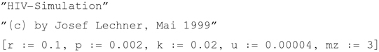
hiv()
Prgm
Ó(c) Josef Lechner, Mai 1999
Ólejos@nol.at
Ó Sequence-Bereich löschen
RclGDB leer
Ó Lokale Variablen
| Local | i,mlist,tlist,asum,astr,aisum,aistr, vsum,vstr,visum,vistr,modus,aktiv,mz |
Ó Definitionen
"1"®mz:2®modus
"0.1"®r:"0.002"®p
"0.02"®k:"0.00004"®u
Define vhsum(mz)=Func
| Local | i,vhsstr |
While iŁmz
If i=1 Then
vhsstr&"u1(n-1)"®vhsstr
Else
vhsstr&"+u"&string(2*i-1)&"(n-1)"®vhsstr
EndIf
i+1®i
EndWhile
vhsstr
EndFunc
Define ahsum(mz)=Func
| Local | i,ahsstr |
While iŁmz
If i=1 Then
ahsstr&"u2(n-1)"®ahsstr
Else
ahsstr&"+u"&string(2*i)&"(n-1)"®ahsstr
EndIf
i+1®i
EndWhile
ahsstr
EndFunc
"Define u"&string(i)&"(n)=when(n=(mdata[2])["&
string((i+1)/2)&"],1,u"&string(i)&"(n-1)+u"&
string(i)&"(n-1)*(r-p*u"&string(i+1)& "(n-1)))"®vstr(i)
"Define u"&string(i+1)&"(n)=u"&string(i+1)&
"(n-1)+k*u"&string(i)&"(n-1)-u*("&vhsum(mz)&")*u"&string(i+1)&"(n-1)"®astr
(i,mz)
"Define ui"&string(i)&"=0"®vistr(i)
"Define ui"&string(i+1)&"=0"®aistr(i)
"Define u"&string(2*mz+1)&"(n)="&vhsum(mz)®vsum(mz)
"Define u"&string(2*mz+2)&"(n)="&ahsum(mz)®asum(mz)
"Define ui"&string(2*mz+1)&"=0"®visum(mz)
"Define ui"&string(2*mz+2)&"=0"®aisum(mz)
Ó
Modell spezifizieren
Dialog
Title "Eingabe
der Modellparameter"
Request "Anzahl
der Mutanden ",mz
Request "Wachstumsr.
Viren r=",r
Request "Aktivitaet
Viren u=",u
Request "Wachs.r.Immmunz.
k=",k
Request "Aktivität
Immunz. p=",p
DropDown "Auftreten
von
Mutanden",{"willkuerlich","schnell","langsam"},modus
EndDlog
Ó
Iterationsgleichungen schreiben
expr(mz)®mz
expr(r)®r:expr(u)®u
expr(k)®k:expr(p)®p
For i,1,mz
expr(vstr(2*i-1))
expr(vistr(2*i-1))
expr(astr(2*i-1,mz))
expr(aistr(2*i-1))
EndFor
expr(vsum(mz)):expr(visum(mz))
expr(asum(mz)):expr(aisum(mz))
Ó
Auftreten von Mutanden steuern
{}®mlist:{}®tlist
If modus=2 Then
500®aktiv
EndIf
If modus=3 Then
4000®aktiv
EndIf
For i,1,mz
augment(mlist,{expr("m"&string(i))})®mlist
If i=1 Then
augment(tlist,{1})®tlist
Else
If modus=1
Then
augment(tlist,{0})®tlist
EndIf
If modus=2
Then
augment(tlist,{rand(aktiv)})®tlist
EndIf
EndIf
EndFor
NewData mdata,mlist,tlist
EndPrgm
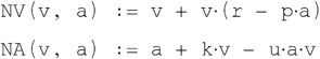
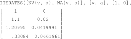
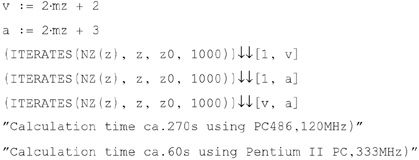
After choosing the
model parameters the iterative equations are defined. NV(v,a) describes
the number of viruses after every step of iteration, VA(v,a) the number
of resistant cells after every step of iteration,
v and
a represent the currently existing viruses and resistant cells
respectively.

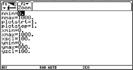
The result of the simulation can be reviewed in the graphic window
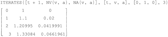
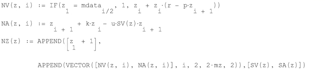
The following three
definitions form the core of the simulation. NV(z,i) calculates the number
of viruses of type i using the current condition z of the system. NA(z,i)
calculates the number of resistant cells against the virus mutant i also
using the current condition z.
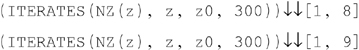
NZ(z) finally
summarizes the iterativ equation for time, all mz iterativ equations for
the respective mutants and the total numbers of viruses and resistant
cells.
Finally a graph of any mutant and any type of resistant cell can be drawn be selecting only two columns.
The same values for the time of appearance of the mutants as for the simulation with the help of the TI-92 have been chosen.
This list should be compiled at random, which can be achieved in the following way:
Literature
| LIPPA, M. (1997): | HIV und Immunsystem - ein mathematisches Modell und seine Realisierung mit EXCEL, MNU 50/5, 295-301 |
| NOWAK, M.A. (1992): | Variability of HIV infections. J. of Theoretical Biology 155, 1-20 |
| NOWAK,
M.A.; MCMICHAEL (1995): |
Scientific American, August 1995. |
| REICHEL, H.-CH. (1999): | Differenzengleichungen in der Oberstufe und ein aktuelles Beispiel über Mathematik und AIDS. To appear in: Didaktik-Reihe der ÖMG. |