Calculating and Presentating 3D-objects with the TI-89/92
With
the TI-89/92 we have a wonderful tool to perform many calculations which
have been preserved for the PC only for a long time. As there is also
a powerful programming and graphing tool available it is a challenge to
combine the calculating and graphing abilities using a program (package).
(You are invited to ask for the package)
We will see
that it is very easy to not only calculate 3D-problems from intersections
of lines and planes through differential geometry in space but also to
illustrate the results by attractivegraphic representations.
We will start with some introductory exercises to get accustomed with my program pres().
Settings: Set your device in Angle mode RADIAN and Exact/Approx AUTO, Switch OFF Axes and Grid in the GRAPH-Window and take care that plots declared in the Y= - Editor might get lost.
Start
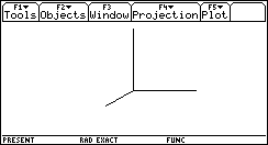
pres() and you will face a newly created menu
bar. The Home Screen is not cleared by the program, because sometimes
you might be glad to refer to your calculations done earlier on the Home
Screen.
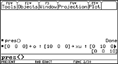
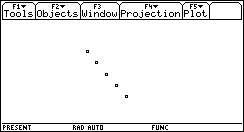
As you can see
on the screen shot, I entered the four points which define the axes. This
way is recommended for later working with the points using variables.
For representation
purpose only you could enter the data points from within the program using
F2 Objects.
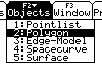

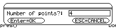
You are asked for an object name: take axes (or any other one of your choice). Then you are asked for the number of points which are necessary to produce axes. Answer with 4.
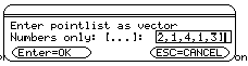
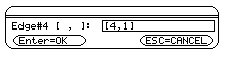
You are asked to enter the four points. You can enter either the variable names of the points (having them defined earlier in the Home Screen) or the coordinates as a vector (between brackets):


[From point#1 to point#2, back to point#1 and to point#4,.....]. So we enter the vector [1,2,1,4,1,3].

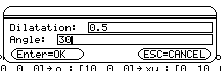
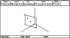
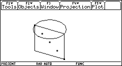
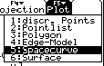
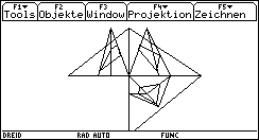
Press F4:Projections and plenty of projections are offered:
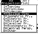
We take dilatation
0.5 and angle 30¯.
Before plotting we have to set appropriate WINDOW-values. It is important to keep in mind the ratio of the graphic windowÇs lengths:
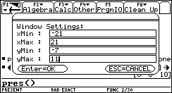
(xMax-xMin) : (yMax yMin) = 7 : 3. DonÇt forget to fix all answers by pressing ENTER.
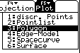
Press F5 Plot and choose option 3:Polygon (because the axes are built as a polygon), and then enter the name of the object.

If we had more objects to represent, then we could add them now.
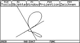
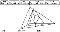
Let the quadrilateral be defined by ABCD [(2,3,0), (4,-3,0), (4,-3,6), (2,3,6)].
Press F2 Objects and then 3:Edge-Model, Name of object: Rect, Number of points: 4. Enter points A through D, point by point:

new object: n.
F5 Plot, 4:Edge-Model, Name of object: rect.
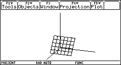
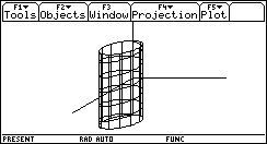
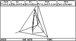
You should see the following figure:
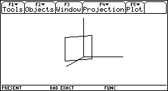
F1 Tools, 1:Clear Screen will clear the screen.
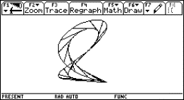
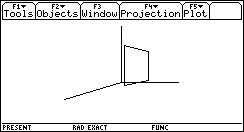
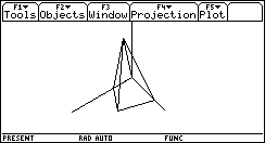
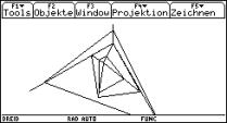
The figure below shows a perspective view.
Leave pres() by F1 Tools, 2:Quit.
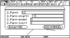
Load pres(). Choose F2 Objects 1:Pointlist.
Name
of object: diago (not diag, because this is an implemented
function)

Then F4 Projections, 5:Isometric and F5 Plot, 1:discr. Points, Pointlist: diago
You should see the 5 points, then add the rectangle rect via F5, 4, rect and the axes (F5, 3, axes)
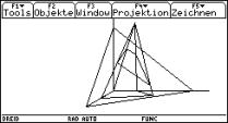
Enter points A through S in the Home Screen. Load pres(), define object "pyra" as a polygon or as list of edges and then you shold find out a nice representation of you pyramid. (eg axonometric proj.).
One possible solution : m = § *(c + d), r = |d c|/2 with C(4,-3,6) and D(2,3,6).
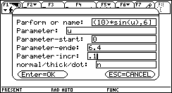
The parameter form of the circle is [3 + r*cos(u), r*sin(u), 6] with r = ø10 and parameter u (0 È u È 2p).
Load pres(), F5 Plot, 5:Spacecurve
You see the circle together with the rectangle and the points from (2) and (3).
Save this plane as parpl, because we will need it in the future.
Choose any projection, define the Window-values and then F5 Plot, 6:Surface
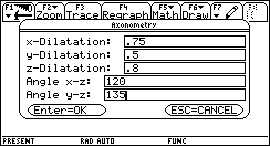
The picture above is in dimetric projection with adjusted Window-values.
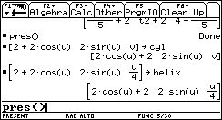
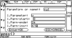
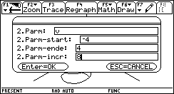
cyl = [2 + 2*cos(u), 2*sin(u), v] with 0 u È 2p; -4 È v È 4
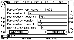
helix = [2+2*cos(u), 2*sin(u), 0.25u] with -16 È u È 16.
You
can easily follow the script. Axes and pyra have been defined in the first
part of this workshop.
So you can skip
repeating this.
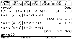
:Enter the given points
C:[3,0,0]£a:[5,5,0]£b:[0,7,0]£c:[0,0,0]£d:[3,3,8]£s
C:[10,0,0]£xe:[0,12,0]£ye:[0,0,8]£ze
:
:The axes:
:
C:[0,0,0]£o:[12,0,0]£xu:[0,12,0]£yu:[0,0,12]£zu
:
:Call pres(), define the pyramid (pyra - pointlist), the plane and the axes.
:
C:pres()
:
:Intersection edges - plane
:
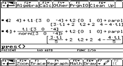
C:p1+t*(p2-p1)£lin(p1,p2)
C:p1+u*(p2-p1)+v*(p3-p1)£pla(p1,p2,p3)
:
C:a+t*(s-a)=xe+u*(ye-xe)+v*(ze-xe)
:
:or
:
C:lin(a,s)=pla(xe,ye,ze)
:
C:rref([0,ˆ10,ˆ10,ˆ7;3,ˆ12,0,0;8,0,ˆ8,0])
:t
= 14/25
:
:with
the TI-92PLUS & 89 it works directly
:
C:solve(3=ˆ10*u-10*v+10
and 3*t=12*u and 8*t=8*v,{t,u,v})
:
C:a+t*(s-a)|t=14/25£a1
:
C:lin(a,s)|t=14/25
:
C:lin(b,s)=pla(xe,ye,ze)
C:b+t*(s-b)=xe+u*(ye-xe)+v*(ze-xe)
C:rref([2,ˆ10,ˆ10,ˆ5;2,12,0,5;8,0,ˆ8,0])
:
C:lin(b,s)|t=5/38£b1
C:b+t*(s-b)|t=5/38£b1
:
:do
the same with SC
:
C:lin(c,s)=pla(xe,ye,ze)
C:c+t*(s-c)=xe+u*(ye-xe)+v*(ze-xe)
C:rref([3,10,10,10;4,12,0,7;8,0,ˆ8,0])
:
:c1
doesn't work, system variable! cc1
:
:
C:lin(c,s)|t=25/58£cc1
C:c+t*(s-c)|t=25/58£cc1
:
C:lin(d,s)=pla(xe,ye,ze)
C:d+t*(s-d)=xe+u*(ye-xe)+v*(ze-xe)
C:rref([3,10,10,10;3,ˆ12,0,0;8,0,ˆ8,0])
:
C:lin(d,s)|t=20/31£d1
C:d+t*(s-d)|t=20/31£d1
:
:
:define
list [a1,b1,cc1,d1,a1] and present it
:
C:pres()
:Definition
of the cone
:Window:
ˆ4 x 10, ˆ3 y 3
:
C:[(3u-3)*cos(v),(3u-3)*sin(v),4u]£cone
:
:0u2
£ double cone; 0u1 £ cone
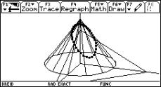
:intersect.pts plane ˆ axes
:
C:[5,0,0]£e1:[0,5,0]£e2:[0,0,3]£e3
:
:define
plane1
:
:{1,2,3,1}£pla1
:
:
C:e3+t1*(e1-e3)+t2*(e2-e3)£pla1
C:pla1=cone
:
C:[[5*t1=3*(u-1)*cos(v),5*t2=3*(u-1)*sin(v),ˆ3*t1-3*t2+3=4*u]]
C:expand(ans(1))
:
:solve
for t1,t2 and u
:
:with
the PLUS we solve the system in one step:
:
C:solve(5*t1=3*(u-1)*cos(v)
and 5*t2=3*(u-1)*sin(v) and ˆ3*t1-3*t2+3=4*u,{t1,t2,u})
:
:[[5*t1=3*u*cos(v)-3*cos(v),5*t2=3*u*sin(v)-3*sin(v),ˆ3*t1-3*t2+3=4*u]]
:
:Put
the equations in the right order and read off the coefficients:
:
C:rref([5,0,ˆ3cos(v),ˆ3cos(v);0,5,ˆ3sin(v),ˆ3sin(v);3,3,4,3])£ell
:
C:ell[4,3]
:
C:cone|u=ans(1)£ellipse
:
C:ellipse
:
:
:present
Objects cone, pla1, ax and ellipse in any projection
:
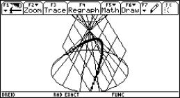
:create a parabolic intersection:
:
:we
shift the cone's base center to
:[4,4,0] £ cone
:
C:[(3u-3)*cos(v)+4,(3u-3)*sin(v)+4,4u]£cone
:
:plane passes [2,2,4] and has direction vectors [3,0,ˆ4]
and [0,1,0]:
:
C:[2,2,4]+t1*[3,0,ˆ4]+t2*[0,1,0]£pla2
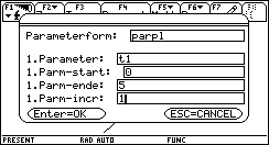
:0.2t11 step 0.2; ˆ1t2 step 1 or use parpl from
(6)
:graph. representation of the plane
:
C:crossp([3,0,ˆ4],[0,1,0])
:
C:dotp([x,y,z],ans(1))=dotp([2,2,4],ans(1))
:intersections with the axes:
:
C:[0,0,20/3]£zs:[5,0,0]£xs
:
C:pla2=cone
C:rref([3,0,ˆ3*cos(v),2-3*cos(v);0,1,ˆ3*sin(v),2- 3*sin(v);
ˆ4,0,ˆ4,ˆ4])£para
C:para[4,3]
C:cone|u=ans(1)£parabel
:
:or
:
C:solve(ans(1)[1,1] and ans(1)[1,2]
and ans(1)[1,3],{u,t1,t2})
C:cone|u=(3cos(v)+1)/(3*(cos(v)+1))£parabel
:
C:zeros(getNum(parabel[1,3]),v)
C:approx(ans(1))
:
:take ˆ1.91 and 1.91 as parameter boundaries
:
:hyperbolic intersection !!?
:
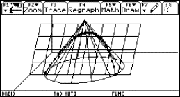
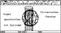
C:[[2*cos(u)+2,2*sin(u),v]]£cyl
:The sphere
C:[[4*cos(u)*cos(v),4*cos(u)*sin(v),4*sin(u)]]
:
:sphere in Cartesian coordinates
C:x^2+y^2+z^2=16|x=cyl[1,1] and y=cyl[1,2] and z=v
C:solve(ans(1),v)
C:cyl|v=2*Ï(ˆ2(cos(u)-1))
C:ans(1)|u=2v
C:ans(1)£viv
C:tExpand(viv)
:[[4*(cos(v))^2,4*sin(v)*cos(v),4*abs(sin(v))]]
:
C:[[4*(cos(v))^2,4*sin(v)*cos(v),4*sin(v)]]£viv
C:tCollect(viv)£viv
:pres()
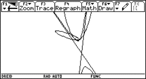
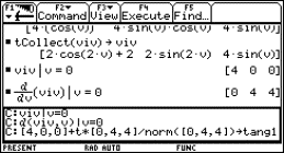
:Tangents in double point (t=0,t=)
C:viv|v=0
C:Ñ(viv,v)|v=0
C:[4,0,0]+t*[0,4,4]/norm([0,4,4])£tang1
C:viv|v=
C:Ñ(viv,v)|v=
C:[4,0,0]+t*[0,4,ˆ4]/norm([0,4,ˆ4])£tang2
:pres()
:
:Surface of tangents
:
C:Ñ(viv,v)
C:viv+u*Ñ(viv,v)/norm(Ñ(viv,v))£tsurf
C:tCollect(tsurf) £tsurf
:pres()
Cylinder:
0 È u È 2p,
-4 È v È 4
Sphere:
0 È u È 2p,
0 È v È p
Space curve viv: 0 È v È 2p
Tangents: -5 È t È 5
Surface of tangents: 0 È v È 2p,
0 È u È 4