Experiences about the use of the symbolic pocket calculator TI-92 in math classes

by Klaus Aspetsberger

Pädagogische Akademie des Bundes in Oberösterreich,

Kaplanhofstraße 40, A-4020 Linz, Austria.

The symbolic pocket calculator TI-92 was used during math lessons at the Stiftsgymnasium Wilhering, a privat high school near Linz in Austria, during the last year. The students were at the age of 17. The different modes of representation (table, graph, algebraic expression) allow to introduce the concepts of calculus in a very natural and illustrative way. In the lecture different possiblities of how to introduce the concepts of analytic geometry and calculus are presented. The TI-92 was also used during tests. We report about the new modified abilities required from the students especially during tests.

Introduction

Since the availability of Computer Algebra Systems (CAS) in the early eighties investigations of how to incorporate these mighty instruments in math courses were undertaken [ ASPETSBERGER, FUNK 1984] . Since the handling of these systems was quite complicated the breakthrough was acchieved by the menu-driven CAS DERIVE in the early nineties. On several national conferences (e.g. [ BÖHM 1992] , [ HEUGL, KUTZLER 1994] ), in the DERIVE Newsletter, the International DERIVE Journal and on two international conferences in Plymouth and Bonn many suggestions for a successful use and results about class room experiments were presented.
In 1996 Texas Instruments presented the pocket calculator TI-92, which incorporates the CAS DERIVE and the interactive geometry package CABRI GEOMETRE. An introduction for the TI-92 and some suggestions for its didactical use can be found in [ Kutzler 1996] , [ ASPETSBERGER, SCHLÖGLHOFER 1996] and [ SCHMIDT 1996] . Due to the availability of pocket calculators doing symbolic manipulations it is possible to introduce CAS in math courses without major organizational problems. The students can use the pocket calculators during math lessons, for doing their home exercizes and for writing tests.
In May 1995 Texas Instruments provided a class of 15 students (12 girls and 3 boys) at the Stiftsgymnasium Wilhering, a privat high school near Linz in Austria, with TI-92 for testing the handling of the TI-92 in real class room situations [ Aspetsberger 1995] . The main points of emphasis of the school lay in teaching languages and the students are mainly interested in arts and languages and not in natural sciences. It was our goal to use the TI-92 for making traditional mathematical contents more illustrative and easier to understand for students.

The experiments are continued and we report in this paper about the experiences of the last school year 1996/97. Now the students were at the age of 17. The math curriculum contains the introduction and application of calculus, non linear analytic geometry, an introduction to probability theory and the treatment of complex numbers. In this paper we only talk about the experiences in calculus and analytic geometry.

Calculus

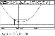
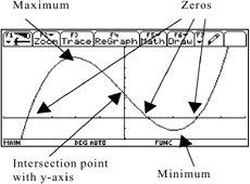
In Calculus we spent much time to introduce the concept of differential quotients solving many problems of various application areas including the tangent problem. Especially for optimization problems the different representation modes of the TI-92 (table, graph, expression) were very helpful for illustration. The students learned how to dedect minima and maxima in tables, graphs and to verify them by means of calculus. For curve analysis the permanent availability of graphs were very illustrative.

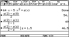
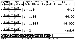
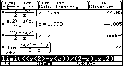
Velocity

We started Calculus by investigating the problem of average and instantaneous velocity. This was an already well known problem for the students and so it was possible to concentrate on the concept of rates of changes and the problem of differentiation. Consider the following typical example. Similar ones can be found in almost all text books for calculus (see for example [ BÜRGER, FISCHER, MALLE 1992] , [ FINNEY, THOMAS, DEMANA, WAITS 1994] )

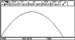
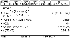
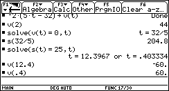
A rock is thrown straight up with a launch velocity of 64 m/sec. It reaches a hight of s(t)=64t-5t² m after t seconds.

Graph the rock`s height as a function of time. Describe the movement of the rock.

Compute the average velocity of the rock within the first two seconds.

Compute the instantaneous velocity after 2 seconds.

Find a general expression for the rock´s velocity after t seconds.

How high does the rock go and when does it reach ist highest point?

How fast is the rock when it is 25 m above the ground?

Having entered the definition for the height s(t) of the rock the students can easily plot the graph of the function. At a first glance we can see, that the rock reaches its highest point after about 8,5 sec in 204 m and returns to ground after about 13 sec.

For computing the average velocity of the rock for the first two seconds we use the formula

, where D s is the change of the height of a body and D t is the time used. For our problem we

enter the expression

The instantaneous velocity after 2 seconds must be slower than the average velocity of the first 2 seconds, because velocity decreases when the rock goes up.

For this reason we compute the average velocity for the time intervals [ 1;2] , [ 1.5;2] , [ 1.9;2] and so on. This can be managed easily by substituting in the general formula for z the starting values of the time intervals.
The students can observe, that the average velocities converge to 44. However, we cannot substitute for z = 2.

Now we use the command limit for computing the limit of

as z approaches 2. At this stage the students had only an intuitive impression of limits, however we can use the TI-92 for computing the limit. We used the command limit as a black box, an exact definition was given afterwards (see for the black box principle [ HEUGL, KLINGER, LECHNER 1996] ).

The students found different definitions for computing the instantaneous velocity by themselves, e.g.

We can take the definitions above to compute the instantaneous velocity of the rock at various times for instance t = 1, 2, 4, 5 and so on. This leads us to generalize the problem and to compute

obtaining an general expression for the velocity of the rock containing the variable t. If we store the expression

to the function v(t) we can easily compute the velocity at any time via a function call.

In the next subproblem we have to find how high the rock goes. In its highest point the velocity of the rock is zero. By solving the equation v(t) = 0 we find out when the rock reaches its highest point. The maximal height can be computed by the function call s(32/5). It was very illustrative to demonstrate the dualism of computing the zeros of v and to find the maximum in the graph.

Finally, in subproblem f) we have to compute the velocity of the rock when it is 25 m above the ground. Again we have to find out the time at first. It was quite surprising for the students to obtain two solutions when we solved the equation s(t) = 25. However using the graph window we saw that the rock is at two moments at a height of 25 m, once when raising up and once when falling down. The negative sign in the velocity of -60 at 24.4 sec indicates the falling process.

Rates of change

In the following we treated many different problems from various application areas ( see [ BÜRGER, FISCHER, MALLE 1992] ). We investigated a reservoir where the content of water decreases according to a certain function V(t), a ballon, which is blown up, and a condensator, which is loaded. All the examples had the same structure and we computed some certain rates of changing.

Finally, we also treated to problem of finding a tangent line to a function graph at a certain point. Determining sequences of secants converging to the tangent line and computing their slopes, the similarity of the examples became visible for the students. For example, it was easy to find the points of a curve, where the tangent lines have a certain slope, especially if the slope is zero.

In the examples above we solved all the problems using the limit command. Thus, the meaning of a derivative of a function was always visible for the students. The TI-92 was used as a calculating aid doing all the complicated computations of the limits.

After introducing the differentiate command the students explored experimentally some simple rules for computing derivatives. It was our goal to concentrate on the meaning of derivatives and we did not train determining derivatives by hand intensively.

Curve analysis

Graphs are very helpful for investigating the behavior of a function. In traditional math courses it was necessary to analyse functions by means of calculus for plotting their graphs. Due to the availability of computers with graphing facilities in math courses the necessity of analysing graphs seems to be superfluous. Indeed we do not need an analysis for plotting the graph, instead of this graph analysis is now important for selecting the interesting intervals of the x- and y-values.
The students were familiar with most of the characteristics of graphs from the need of documenting graphs in their exercise notebooks, because to draw the graphs exactly would cancel out the advantage of plotting the graphs by the TI-92.

So the students had to give a rough sketch containing the characteristics of the graph. The students had to decide for each problem the typical aspects and the range for the x-values which was important. However, in most cases it was sufficient to mark zeros, maxima and minima of the graph and to add the coordinates of these characteristic points to the sketch.
The necessity of figuring out the essential features of graphs turned out to be very helpful for dicussing graphs by means of calculus. The students were familiar with most of the concepts of curve analysis.[ ASPETSBERGER, FUCHS 1997] . New was the treatment of the end behavior of polynomial functions and how to dedect minima and maxima by the means of calculus.

We demonstrated that it is impossible to find out the end behavior of polynomials from the small picture presented in a graph window. We plotted several polynomial functions which have similar graphs in a standard plot window but different end behaviour.

Graphing many polynomial functions the students discovered the rule of how the end behavior depends on the degree of the polynomials.
The students were already familiar with minima and maxima from documenting graphs. They were also aware that minima and maxima have tangent lines with a slope 0, however we had to discuss the coherence to the second derivative. The possibility of simultaneously plotting of a function, its first and second derivative was very illustrative and helpful for understanding these correlations.

Rational functions

Discussing rational function we can use the TI-92 also for introducing mathematical concepts (see also [ Aspetsberger, Fuchs, Klinger 1994] , [ HEUGL, KLINGER, LECHNER 1996] ). According to polynomial functions there are two new aspects arising when treating rational functions. The first one is, that rational functions are not defined at the zeros of the denominators. These values of x and the corresponding vertical asymptotes can be found in the graphs easily.

The second aspect are asymptotes describing the end behavior of the functions for very large or very small x-values. The concept of asymptotes can be developed experimentally.
In the following example we investigate the graph of the rational function

. If we zoom out several times we can see that the graph of the function looks like a straight line. This means that a linear function is a good approximation of the end behavior of the rational function.


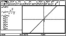
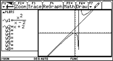
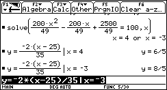
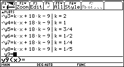
Now we have to find a suited linear function fitting well to the rational function. By inspection of the graph we suggest that the slope of the linear function should be k = 1. Our first guess is y2(x) = x.

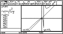
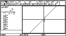
Zooming in we see that the graph of the function y2(x) lies beyond the graph of y1(x). By trial and error we find the suited expression y2(x) = x+2.

Now we try to verify the suggestion that y2 is a good approximation of y1 for large x-values. A first attempt could be to inspect a table where we compute the differences of y1(x) and y2(x). Of course this is not a proof, because we are evaluating some sample points only. However, we get an idea of how to define the concept of an asymptote of a rational function.

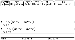
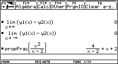
For an algebraic investigation we compute the limit of the difference of the rational function

, which we have stored to the internal function y1(x), and the linear function x+2, which we stored to y2(x). Both limits for very large and very small x-values are zero.

In the example above we have found the asymptote experimentally. For complicated rational functions this could be rather difficult. How can we determine an asymptote algebraically? Consider the following polynomial division of the rational function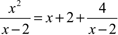

. The quotient x+2 is the asymptote of the rational function, since the remainder

of the polynomial division converges to zero for very large or very small x-values.

In the lessons we applied the experimental method above also for asymptotes of degree 2. However it was neccessary, that the students were able to find the defining expressions of quadratic functions when the graphs were given [ ASPETSBERGER, FUCHS 1996a] .

Analytic Geometry

The introduction and analysis of ellipses, parabolas and hyperbolas are the topics of analytic geometry for students of the eleventh form at Austrian high schools. We started with a short repetition of circles and a recapitulation of the techniques of how to plot circles in graph windows. We discussed two methods for plotting circles.

Circles

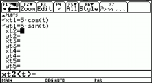
For plotting a circle with midpoint M(0/0) and radius r=5 we first solve the equation of circle x²+y²=25 according to the variable y. Since we want to illustrate different graphs and curves simultaneously, we store the two branches of the circle to the internal functions y₁(x) and y₂(x).

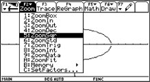
In the graph window the two branches of the circle are plotted. There are little holes in the circle at the x-axis. Due to different scales of the x- and the y-axis the circle appears as an ellipse. With the command ZoomSqr of the Zoom-menue appropriate settings for the x- and the y-axis are selected automatically to obtain correct circles or squares.

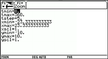
The second method was to plot the circle as a parametric function. Therefore we have to define parametric functions for the x-coordinates and for the y-coordinates of the points lying on the circle. The parameter must be called t. If we choose appropriate settings for the window we obtain the image of a circle without holes.

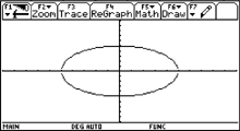
The students prefered the first method, since most of our functions were defined without parameters.
The disadvantage of plotting an ellipse instead of a circle with the standard settings of the TI-92 was used as a starting point for introducing and discussing ellipses.

Ellipse

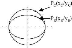
Due to the different scalling factor of the x- and y-axis a circle looks like an ellipse. The circle is squeezed in direction of the y-axis. In the figure beside a circle and its correspondent ellipse are presented. The point P_C of the circle with the coordinates P_c(x_c/y_c) is moved to the point P_E of the ellipse with the coordinates P_E(x_E/y_E). As the point is only shifted in direction of the y-axis the x-coordinates of the points are equal x_c=x_E. However for the y-coordinates the proportion y_E:y_c=b:a is true, where a is the radius of the circle and b half of the diameter of the ellipse in y-direction. So we can derive the following equality for the y-coordinates of the points of the circle

. If we substitute these relations for the coordinates of the circle points into the equation of the circle x²_c+y²_c=a², we obtain the following relation for the coordinates of the points of the ellipse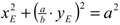

, which can be easily transformed to the equation of an ellipse b²x²+a²y²=a²b².

It was quite easy for the students to understand this derivation. Later on we also introduced the focus points of an ellipse and proved the relation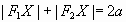

of the ellipse points X to the focus points F₁, F₂, which is commonly used for defining ellipses [ REICHEL, MÜLLER, HANISCH, LAUB 1992] . We used this definition when working in the interactive geometry window of the TI-92.

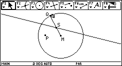
We start our construction with a circle, a point P within the circle and a point Q on the circle. Now we draw a segment from the point Q to the midpoint M of the circle. Finally, we determine the intersection point S of the perpendicular bisector of P and Q with the segment from Q to M.

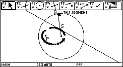
Now we move the point Q along the circle tracing the places of intersection point S. The locus of S according to Q on the circle is an ellipse. We can do this stepwise by the Trace command which is very illustrative or in one step by the command Locus. There is also the possibility of doing an animation.

In class we presented the construction and the students had to find out, why all these points lie on an ellipse. The ideas of the constrution follows a suggestion from Franz Schlöglhofer.
The advantage of this construction is, that it is very simple. This circumstance is very important, because complicated constructions sometimes require nearly whole time of a lesson and there is no further time for experimenting or argueing. In [ Weigand 1997] a couple of simple constructions are presented for experimenting with interactive geometry programms.

If we trace the location of the perpendicular bisector, we see, that the bisectors are tangent lines of the ellipse. The task of the students was, to find out, how to construct a tangent to an ellipse in an arbitrary point of the ellipse.

Intersection points

The next technique is how to determine the intersection points of an ellipse with other curves. Consider the following example:

Determine the intersection points of the ellipse 4x²+25y²=100 and the straight line 2x+35y=50 !

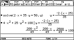
First we have to express the variable y from the straight line explicitly. Substituting this expression into the ellipse we obtain an equation in the variable y solely. Solving this equation according to x we obtain the x-coordinates of the intersection points. Finally, we have to substitute these results into the equation of the straight line. Problems may occur, if the students substitute the results into the equation of the ellipse, which would not lead to unique solutions.

For illustration the students can store the two branches of the ellipse and the explicit expression of the straight line to the internal function y1(x), y2(x) and y3(x) and to plot them in a graph window.

Here the students can verify their results.

Tangent lines

The last problem is to find tangents to an ellipse. The method we used in the course was both suited for determining tangents through points on the ellipse or lying outside of the ellipse. Consider the following example:

Find the tangent line to the ellipse x²+2y²=54 through point P(-18/-9) outside of the ellipse! (see [ REICHEL, MÜLLER, HANISCH, LAUB 1992] , p.192)

First we enter the general form of the tangent line with the unknown parameters k and d. For determining d we substitute the coordinates of P, because the tangent line is running through P. Solving the expression -9=d-18*k according to the variable d we obtain d=18*k-9 which we can subsitute in the general form of the tangent line. y=k*x+18*k-9 is the general form of a straight line trough point P.

As an experimental attempt we can plot the ellipse and try to find tangent lines by varying the slope k of the straight lines. Similar to circles we obtain straight lines that have one, two or no points in common with the ellipse. Obviously, the straight lines with only one intersection points are tangents.

This definition leads us to a method of how to determine tangent lines. Our plan is to determine the intersection points of the general form of a straight line through P with the ellipse. These solutions x₁ and x₂ still depend on the parameter k which is the slope of the straight line. Since tangent lines have only one intersection point with the ellipse we solve the equation x₁=x₂ for determining the slopes of the tangent lines.

First we substitute the general form of the straight line through P into the equation of the ellipse obtaining an equation with the variables x and k. Solving this equation according to the variable x we obtain the x-coordinates of the intersection points.

Solving the equation x₁=x₂ according to k we determine the slopes of the tangent lines which we can substitute into the general form of the straight lines to obtain the tangents.

These expressions and equations are quite bulky. However, the power of the computer algebra systems helps to solve the equations and to manage substitution and simplification of the expressions. The task of the students is to organize the problem solving process.

The method described above for determining tangent lines is not new. In traditional courses, i.e. math courses without using computer algebra systems, equations like d²=a²*k²+b² are derived in general, providing a relation between the parameters of the ellipse a and b and the parameters of the tangents k and d. This relation seems to be easier than the expressions we have deduced. However, once the formula is derived the process of making two intersection points unique is invisible and so many students use the formula above as a black box without understanding its meaning. Using a computer algebra system the students always have to be aware of what happens at the moment.

Parabolas

A main advantage of the method described above is that we can use it for computing tangents to hyperbolas and parabolas too. Hyperbolas and parabolas are open curves. Thus, it is not totally clear, whether a line with only one intersection point is a tangent. Consider the following example:

Find a tangent line for the parabola y²=48x running through the point S(-6/6), which lays outside of the parabola. ([ REICHEL, MÜLLER, HANISCH, LAUB 1992]

Similar to the expample above we compute a general form y=kx+6k+6 of a straight line running through S with a variable parameter k. Next we determine the intersection points of this straight line with the parabola solving the equation (kx+6(k+1))²=48x according to the variable x.

We obtain two solutions for x depending on
the variable k and

. For determining a suitable k, we solve the equation x₁ = x₂ according to the variable k making both intersection points unique. Finally, we have to substitute the solutions k = 1 or k = -2 into the general form of the straight line above to obtain the expressions of the tangent lines.

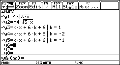
For illustration we determine both branches of the parabola and store the results to the internal functions y₁(x) and y₂(x). The two expressions of the tangent lines are stored to the functions y₃(x) and y₄(x). Now we can plot the parabola and the tangent lines in one graph window simultaneously.

Choosing suitable parameters for the coordinate system we can inspect the parabola and both tangent lines in the graph window.

Now one can suppose that there are also straight lines that are not tangent lines and have only one intersection point with the parabola in common. For instance, if we choose a straight line with a parameter k = -1, we obtain a straight line which is not a tangent line and has only one intersection point with the parabola.

This example seems to be a contradiction to the definition of tangent lines above.

However, if we substitute in the home window for k=-1 within the general solution for the intersection points above we obtain two different intersection points. The first one at x=0 can be seen in the graph window. The second one at x=48 is invisible due to inappropriate window settings [ ASPETSBERGER, FUCHS 1996b] .

For visualization of the second intersection point we change the settings for the x-axis to

and choose appropriate settings for the y-axis.

Now the students can find out experimentally, that for all k with -2<k<1 except k=0 all straight lines through S(-6/6) have two intersection points with the parabola. This is due to the fact, that the gradient (slope) of the parabola decreases for increasing x-values, whereas the slope of a straight line is constant for all x. The circumstance that the gradient of a parabola converges to zero for increasing x-values can be verified be means of calculus.

Experiences

One of the main advantages of the TI-92 are the different forms of representation (tables, graphs, expressions) which are always available on the TI-92 and can lead to a better understanding of mathematical concepts. The students have the possibility to choose a representation form they like most e.g. for solving problems, for illustration or to get an overview in a certain situation. It is remarkable, that most students choose tables or graphs to solve problems, if the method is free. Only very few students use expressions for solving problems or for illustration. The abstractness of expressions is a major handicap in traditional math courses when introducing new mathematical concepts. So the availability of different representation forms helps to differentiate and individualize the prozess of math teaching.

The use of a CAS or the TI-92 in special requires to learn techniques. There are techniques for the handling of the TI-92, e.g. for plotting graphs, for changing the window settings, for computing tables. On the other hand students have to obtain abilities that are independend of the CAS used. They have to learn how to document their results concentrating on the essential points. This is very important for sketching graphs and tables. However, the problem occurs also when documenting algebraic transformations. It is not possible on the TI-92 to plot the expressions of a home window directly. So the students have to recognize and to write down only the important steps. Documenting results is very important when using the TI-92 for tests. We had to find modes of how to document calculation steps sufficiently. This was quite a difficult task, since it was not possible to give definitions of "essential", "sufficient" or "important". Documenting results and retaining the overview during calculation were the two most important abilities the students had to learn when using CAS during tests.

The learning of all these techniques required time. However these techniques seemed to be so important that they warrant the additional amount of time. On the other hand we saved time since we did not have to train techniques for transforming expressions, solving equations, computing derivatives etc.

The CAS is able to handle all the computing problems. It is not neccessary to find tricky ways for solving problems. Introducing new concepts we can start with very elementary and - due to that reason - very illustrative methods. For instance, we solved most problems of calculus using the limit of the quotient of differences. Therefore the students got a better understanding of the concept of a differential quotient and of derivatives. The problem of computing the limits was dedicated to the computer.

Due to the availability of the computational power of a CAS it is not neccessary to treat techniques, e.g. for solving complicate equations, doing complex derivatives or computing limits, in advance. There is always the possibility of verifying important steps afterwards. Then the students knew the connections and are more motivated for doing an abstract proof.

The possibility of recovering mathematical contents experimentally is very motivating for many students. The use of a computer gives many opportunities for experiments. However, experiments are quite time consuming and some students prefer traditional methods, because they are more convenient for them.

References

[ ASPETSBERGER, FUNK 1984]
Aspetsberger K., Funk G.: Experiments with muMATH in Austrian High Schools, in Buchberger (ed.) Proc. ICME´5 Conference, technology theme, Adelaide, Australia, August 24-30, 1984.

[ ASPETSBERGER, FUCHS, KLINGER 1994]
Aspetsberger K., Fuchs K., Klinger W.: Derive - Beispiele und Ideen. Zentrum für Schulentwicklung, Klagenfurt, 1994, ISBN 3-9500283

[ ASPETSBERGER 1995]
Aspetsberger K.: Schulversuch. TI-Nachrichten für die Schule, Informationsservice des Bereichs Personal Productivity Products, Texas Instruments, Ausgabe 2/95

[ ASPETSBERGER, FUCHS 1996a]
Aspetsberger K., Fuchs K.: Computer Algebra Systeme für den Mathematikunterricht. Praxis der EDV/Informatik, Verlag Jugend & Volk.

[ ASPETSBERGER, FUCHS 1996b]
Aspetsberger K., Fuchs K.: DERIVE und der Rechner TI-92 im Mathematikunterricht der
10. Schulstufe. International DERIVE and TI-92 Conference, Computeralgebra in Matheducation, Bonn 1996.

[ ASPETSBERGER, SCHLÖGLHOFER 1996]
Aspetsberger K., Schlöglhofer F.: Der TI-92 im Mathematikunterricht, Texas Instruments, 1996

[ ASPETSBERGER, FUCHS 1997]
Aspetsberger K., Fuchs K.: Lehrerausbildung und Mathematikunterricht mit dem Symbolrechner
TI-92. In: Beiträge zum Mathematikunterricht 1997, Verlag franzbecker. 31. Tagung für Didaktik der Mathematik, Leipzig, März 1997.

[ BÖHM 1992]
Böhm J. (editor): Teaching Mathematics through DERIVE. Proceedings of Krems´92 Conference, April 27-30, 1992, Krems, Austria, Chartwell-Bratt, Bromley/UK, 1992

[ BÜRGER, FISCHER, MALLE 1992]
Bürger H., Fischer R., Malle G., Kronfellner M., Mühlgassner T., Schlöglhofer F.: Mathematik Oberstufe 3, Hölder-Pichler-Tempsky, Wien, 1992.

[ FINNEY, THOMAS, DEMANA, WAITS 1994]
Finney R.L., Thomas G.B., Demana F.D., Waits B.K.: Calculus: graphical, numerical, algebraic. Addison-Wesley, 1994.

[ HEUGL, KUTZLER 1994]
Heugl H., Kutzler B. (editors): DERIVE in Education -Opportunities and Strategies. Proceedings of the Krems´93 Conference, Sept. 27-30, 1993, Krems, Austria, Chartwell-Bratt, Bromley/UK, 1994

[ HEUGL, KLINGER, LECHNER 1996]
Heugl H., Klinger W., Lechner J.: Mathematikunterricht mit Computeralgebra-Systemen (Ein didaktisches Lehrbuch mit Erfahrungen aus dem österreichischen DERIVE-Projekt). Addison-Wesley, Bonn, 1996.

[ KUTZLER 1996]
Kutzler B.: Symbolrechner TI-92. Computeralgebra im Taschenformat. Addison-Wesley, Bonn, 1996

[ Reichel, Müller, Hanisch, Laub 1992]
Reichel H.C., Müller R., Hanisch G., Laub J.: Lehrbuch der Mathematik 7, Hölder-Pichler-Tempsky, Wien, 1992.

[ SCHMIDT 1996]
Schmitdt G.: Mathematik erleben mit dem TI-92, Texas Instruments, 1996

[ WEIGAND 1997]
Weigand H.G.: Computer - Chance und Herausforderung für den Geometrieunterricht. Mathematik lehren, Ernst Klett Verlag, Nr. 82, Juni 1997.